Walmart's 1.5M-Square-Foot New York Fulfillment Plan: How to Model Regional Warehouse Capacity

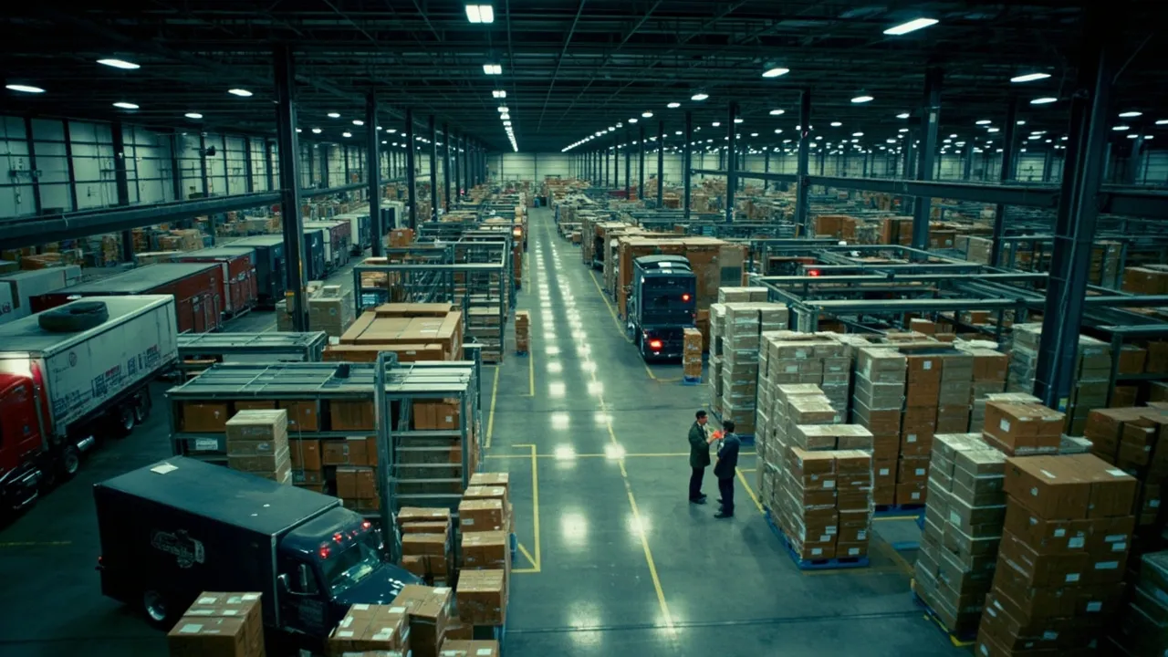
Walmart's proposed fulfillment warehouse in New York is enormous even by modern logistics standards. The retailer filed plans in July for a roughly 1.5 million-square-foot facility in Wallkill, Orange County, according to Supply Chain Dive. The proposal includes truck courts and loading areas, placing transportation capacity at the center of the site's design rather than treating it as a downstream concern.

For logistics teams, the useful question is not whether their next facility should match Walmart's scale. It is how to translate any large footprint into defensible operating assumptions. Square footage alone does not reveal how many orders a building can ship, how many trailers it can turn, or whether labor and carrier capacity can absorb a peak week.

The answer is a regional warehouse capacity model connecting space, inventory, work content, dock flow, and transportation demand. Every assumption should be expressed as a range and tested against a peak scenario before a company commits capital or inventory.

Start with usable space, not the headline number

A 1.5 million-square-foot building does not provide 1.5 million square feet of storage. Receiving, shipping, staging, returns, value-added services, battery charging, maintenance, offices, fire lanes, and automation equipment all consume space.

A first-pass model might assign 55% to 65% of the building to storage and reserve the rest for movement and support functions. At 60%, the Wallkill-scale example would yield 900,000 square feet of storage area. That is a planning scenario, not a disclosed Walmart specification. The correct percentage depends on product dimensions, storage media, automation, fire code, and the amount of inbound and outbound staging required.

Convert that area into effective storage positions by product family. Pallets, cases, each-pick inventory, oversize goods, and hazardous materials have different space and handling requirements. Then apply an operating occupancy ceiling. Designing around 100% utilization is a trap: when every slot is full, replenishment slows, putaway queues grow, and workers spend more time searching for exceptions.

Translate order demand into hourly throughput

Annual unit volume hides the pressure that determines facility size. Build the capacity model from the busiest credible week, day, and hour.

Suppose a planning scenario calls for 200,000 outbound order lines on a peak day over two effective 10-hour shipping shifts. That requires an average of 10,000 lines per hour. If a two-hour carrier cutoff window concentrates 30% of demand, however, the operation must process 30,000 lines in that window, or 15,000 per hour. The higher requirement governs the labor, sortation, staging, and dock plan.

Model each process separately:

• Receiving capacity by pallets or cases unloaded per labor-hour.
• Putaway and replenishment moves by storage zone.
• Pick rate by unit, case, pallet, and automation path.
• Pack and sort rate by order profile and destination.
• Staging dwell between shipment completion and trailer departure.

The weakest stage sets building throughput. Adding pick capacity accomplishes little if outbound staging fills before trucks arrive.

Make dock demand a timed calculation

Dock-door counts are often copied from a comparable building or expressed as doors per square foot. A stronger model calculates concurrent demand.

For each hour, estimate inbound appointments, outbound departures, average door occupancy, live-load versus drop-trailer share, and a disruption allowance. If 24 outbound trailers must depart during a two-hour peak and each occupies a door for 75 minutes, the base workload is 30 door-hours. Dividing by two hours implies 15 doors continuously occupied. Applying a 20% recovery allowance raises the requirement to 18 doors before adding inbound activity.

That example is illustrative, but the method exposes the real constraints. Late arrivals, paperwork holds, pallet rework, seal discrepancies, and missing drivers consume dock capacity even when the warehouse itself is productive. The appointment system must therefore exchange planned arrival, check-in, door assignment, loading start, loading completion, and departure events with the TMS and WMS.

Model labor as work content, not headcount

Large buildings can obscure labor problems because employees are distributed across long travel paths and multiple process areas. Calculate labor from forecast transactions multiplied by standard minutes per task. Add indirect work, breaks, training, supervision, maintenance, and realistic absence assumptions.

Run at least three scenarios: base demand, seasonal peak, and disrupted peak. The disrupted case should combine elevated orders with reduced productivity, a late inbound wave, or constrained carrier availability. If a design works only when every process achieves engineered rates simultaneously, it has no operational resilience.

Warehouse demand indicators also provide context for the decision. Logistics Management reported a Q2 Prologis Industrial Business Indicator Activity Index reading of 59.3, within a sustained 55-to-60 range associated with improving demand. External indexes should inform a forecast, but they cannot replace the company's own order, inventory, and shipment history.

Compare inventory savings with parcel and replenishment costs

A Northeast node can shorten customer distance and reduce parcel zones, but it also divides inventory across more locations. Slow-moving items may require additional safety stock, while fast sellers benefit from proximity to demand.

Compare network scenarios using total landed cost and service, including:

• Parcel or final-mile cost by destination ZIP code, weight, and package dimensions.
• Inbound replenishment cost and lead time from suppliers or upstream distribution centers.
• Inventory carrying cost, safety stock, obsolescence, and transfer expense.
• Facility, automation, labor, utilities, and local tax assumptions.
• Expected delivery promise, cutoff time, and peak capacity by region.

Test a centralized network, a regional node with all stock-keeping units, and a regional node carrying only high-velocity inventory. The selective model often deserves special attention because it captures much of the parcel benefit without duplicating the entire assortment.

Build the decision from shared TMS and WMS data

Before approving a regional node, planners need order lines and cube by destination, SKU velocity and seasonality, inbound origins, shipment lead times, carrier performance, parcel-zone costs, appointment history, trailer dwell, and labor standards. The records must share identifiers and timestamps so an order forecast can be translated into inventory moves, dock appointments, and carrier tenders.

Once the building opens, preserve the assumptions as operating targets. Compare forecast versus actual order profiles, labor minutes, dock occupancy, tender acceptance, and cutoff attainment. When demand changes, the model becomes an early-warning system rather than a forgotten capital-project spreadsheet.

CXTMS connects orders, appointments, inventory-related shipment plans, carrier capacity, and execution milestones so teams can test and operate regional networks with the same data. Request a CXTMS demo to see how transportation visibility turns warehouse capacity assumptions into a measurable fulfillment plan.