Peak Season Ends Unevenly: Plan the Import Drop by Gateway, Not National Average

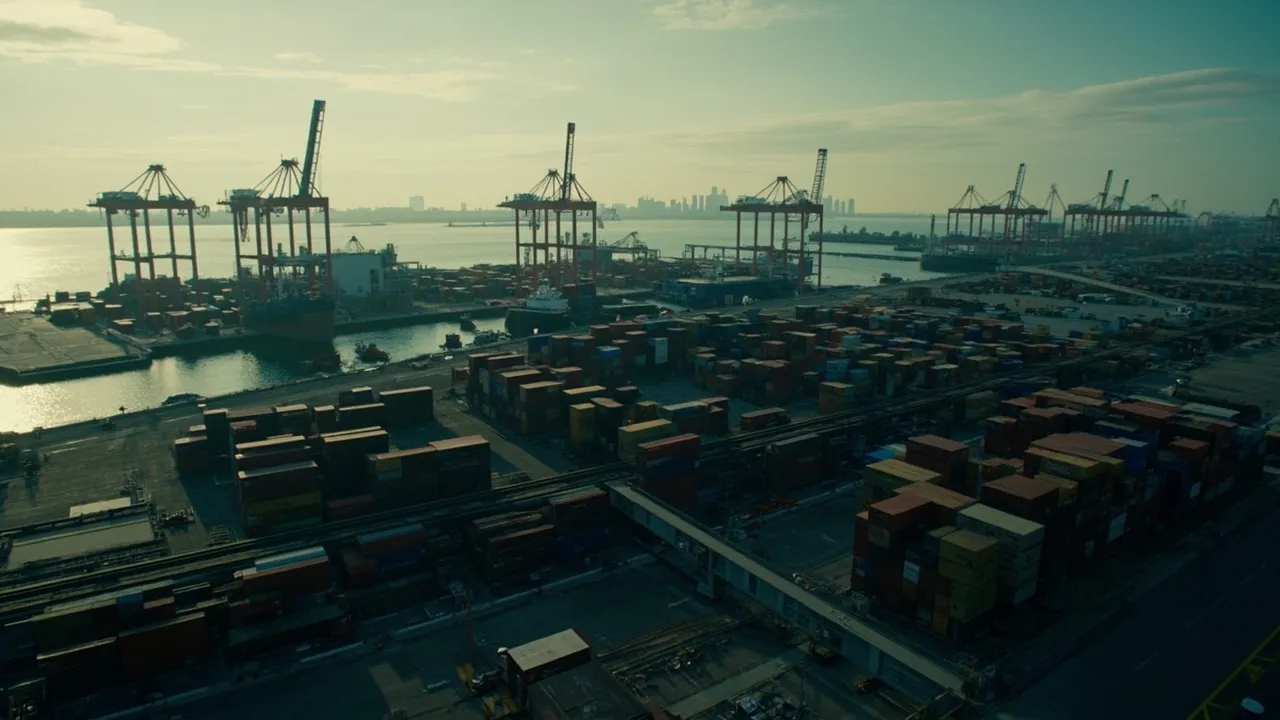
The extended U.S. import peak is winding down, but it is not ending at the same speed everywhere. That distinction matters for importers deciding when to release drayage capacity, warehouse labor, rail reservations, and overflow storage.
The latest Global Port Tracker outlook expects imports at major U.S. container ports to decline through the balance of 2026. Yet the national direction does not describe the workload facing an individual terminal or distribution center. In August, ports covered by the report handled 2.3 million TEU—down 0.7% from a year earlier but up 0.4% from July, according to Logistics Management. A market can be declining year over year while still creating a sequential operational peak.
That is why a single demand haircut across every gateway is the wrong response. Import planning should start with each port's release curve and the downstream capacity needed to clear it.
A national forecast does not move a container
National TEU totals are useful for budgeting and market context. They are less useful for deciding how many drivers to schedule Tuesday morning at Savannah, how much rail capacity to retain from Los Angeles, or whether a New Jersey warehouse can release weekend labor.
Several local variables can diverge from the headline:
- Vessel bunching: Two late sailings can arrive together even when the month's total volume is lower.
- Terminal dwell: Congestion, inspection holds, chassis availability, and appointment limits determine when boxes become collectible.
- Rail departures: A gateway may discharge containers normally while missed train connections expand the on-dock inventory.
- Warehouse carryover: Facilities can remain full of earlier peak-season receipts, reducing capacity for a smaller inbound wave.
- Import mix: A decline in discretionary retail freight does not necessarily reduce temperature-controlled, time-sensitive, or project cargo at the same rate.
Ocean pricing reinforces the point. Supply Chain Dive reported that Asia-to-U.S. West Coast spot rates fell just 1% as of November 10. A slight rate move is evidence of easing, not proof that every gateway has excess capacity ready to release.
Build one scenario set for each gateway
For every major port in the network, planners should maintain three rolling scenarios: expected, delayed-release, and concentrated-arrival. Each scenario should cover the full chain from discharge to final warehouse receipt.
Start with containers expected to become available—not simply vessels expected to arrive. Apply terminal-specific assumptions for discharge time, customs or agency holds, free time, appointment availability, and historical no-show rates. Then convert the release curve into daily drayage moves.
Next, map those moves to storage and labor. Measure warehouse capacity in usable receiving slots, not nominal square footage. A building may appear to have space while labor, dock doors, or putaway locations are already committed. Include inventory left from the extended peak and identify the date when each block of capacity actually becomes reusable.
Finally, align rail and truck reservations with the same daily curve. The result should be a gateway plan that answers four practical questions:
- How many containers can become available each day?
- How many can the transport network remove before free time expires?
- How many can the destination receive without creating yard or floor congestion?
- What recovery option remains if the forecast is wrong?
The national forecast can inform the expected case. Local operating data must determine the delayed and concentrated cases.
Return capacity in stages, not all at once
Reserved capacity carries a cost, so holding every peak-season commitment indefinitely is not sensible. Releasing it too early can be more expensive once demurrage, detention, spot drayage, overtime, and missed rail connections are included.
Use staged return triggers instead of a calendar date. For example, release the first block of flexible drayage capacity only when the gateway's seven-day available-container forecast falls below 85% of committed pickup capacity. Release a second block when actual terminal availability stays below 75% for two consecutive weeks and warehouse receiving utilization remains below 80%.
Protect a smaller recovery block until the risk window closes. That block might include weekend driver coverage, an overflow yard, additional receiving shifts, or the right to restore rail allocation. Its release should depend on leading indicators such as vessels within seven days, containers on hold, terminal dwell, appointment fill rates, and warehouse backlog—not merely the number of containers already received.
Thresholds will differ by gateway. A port with reliable appointments and nearby overflow storage can operate with a thinner buffer. A gateway dependent on limited rail departures or a tightly scheduled distribution center needs more recovery capacity.
Put gateway signals in one operating view
The planning process breaks down when ocean teams track vessel schedules, drayage teams track appointments, and warehouses track labor in separate files. By the time the data is reconciled, the opportunity to return or restore capacity may have passed.
A transportation management system should connect booking, estimated arrival, discharge, availability, appointment, pickup, rail departure, and delivery milestones. Pair those events with capacity commitments and costs. Planners can then compare the national outlook with actual gateway conditions and see whether a decline is flowing through the network—or simply waiting at a different node.
The end of peak season should reduce cost and pressure. It should not create a new service failure because capacity was withdrawn according to an average that no individual gateway experienced.
Ready to plan import capacity around real gateway events? Request a CXTMS demo and see how one operating view can connect port milestones, reservations, exceptions, and recovery decisions.